Introduction

This is not the first time I try to look into getting a color in a cell when the value of the cell is such and such, not just smaller than 0 and it becomes [RED]... which is a default available in your formula.

The fact is that you need to create styles that you're going to reference either with the STYLE() function or using the Conditional Formatting window.

So...

P.S. This is only available in Calc.

Creating New Styles and Formatting

First select a cell. You probably want to use an empty cell where you can enter a number or some text and then change it's format with the Format Cell... option. Once that is done, you can drag and drop the cell on the Styles and Formatting window and name it. That name is what you will use to format a cell dynamically.

1. Click on an empty cell
2. Enter the word "Test"
3. Right click and select Format Cell...
4. Change the formatting to your liking
5. Once setup, click OK
6. If it still looks wrong, repeat steps 4 and 5
7. Hit the F11 key once to open the Styles and Formatting window (You can also use the View » Styles and Formatting menu.)
8. Click once on the cell you just formatted (it should already be selected, though)
9. Click and hold the left mouse button down
10. Drag the cell to the Styles and Formatting window
11. Release the mouse button, a popup window opens
12. Enter a name (i.e. "My Favorite Color") and click OK

Now you see your new style appear in the list.

If you need multiple formats, create others now. For example, you may want a green color if the value is more than $10,000 and a red color when under $5,000. In such a case you need two styles: a red style ("Too Small") and a green style ("Perfect").

Dynamically Setting Up the Cell Format

Now we're ready to set the cell format.

There are two ways of doing it: using the STYLE() function which means you can do that within the cell formula, or using the Conditional Formatting window.

Using the STYLE() function with numbers

Say you want the value to go to "Too Small" when under $5,000. Your cell formula will look like this:

=SUM(A1:A20)+STYLE(IF(CURRENT()<5000,"Too Small","Default"))

The CURRENT() function is used to test the value in the current cell. You could reference another cell too, i.e. if the cell above is too small, then this cell will use the "Too Small" format.

Note that the STYLE() function accepts three parameters. The first one is expected to be the name of the style to use on load or whenever a new computation goes on. The second parameter is a number of seconds to hold that value. The third value is the name of another style to use after that number of seconds passed.

STYLE(start-style, time-seconds, final-style)

This method allows you to easily copy the STYLE() function from one cell to another.

Using the STYLE() function with text

Whenever you create a cell with text instead of numbers, you need to transform the style in a string which is done with the T() function.

So for example:

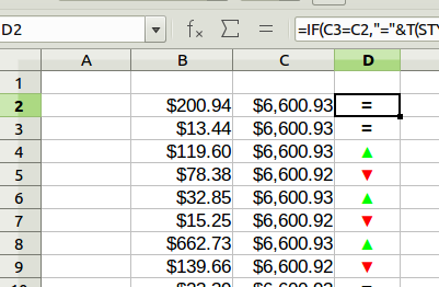
=IF(C3=C2,"="&T(STYLE("EqualStyle")),
          IF(C3>C2,"▼"&T(STYLE("RedStyle")),
                   "▲"&T(STYLE("GreenStyle"))))

Here I check two values from the next cell and the current cell. If they are equal, put an equal sign and use the EqualStyle.

If the next value is larger, then use a down arrow and show it in red.

If the next value is smaller, then use the up arrow and show it in green.

This works because the STYLE() function returns the number 0.

Conditional Formatting

The other method may be easier for you to use. Instead of entering the style in the formula, you use a popup window found in Format » Conditional Formatting » Condition menu.

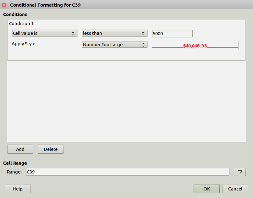
In the example above, I selected "Number too Large" and the format shows the number in red when that happens. The limit is set to $5,000. Just check out the various dropdowns to change the condition as required.

You can Add more than one condition and you can select multiple cells to setup that format (see the Cell Range line). Use the Delete button to remove a condition. Once done click OK.